Day 1 with nflfastR

Sports have been a huge part of my life since pretty much forever. I collected sports cards as a kid and played just about every major sport competitively through high school. There's almost nothing that I love more than sports and it has always been a dream of mine to work in the industry professionally.

What's interesting is that I currently work as a Sr. Talent Partner at one of the best tech companies in the world, Adobe! Talent Partners for the most part are considered non-technical people, so for me to embark on a journey to learn R is somewhat unheard of for someone in my profession. But I am not your typical recruiter, mwahaha.

What started off as an exploration snowballed into the creation of a full-blown Shiny dashboard that I developed from scratch which displays important recruiting metrics globally across the Adobe Talent Acquisition (TA) team. After learning the basics of R, Shiny, and ggplot2 I figured it wouldn't be too difficult to get started with looking at sports data. After doing some research I came across the nflfastR package.

nflfastR is a set of functions to efficiently scrape NFL play-by-play data. nflfastR expands upon the features of nflscrapR: The package contains NFL play-by-play data back to 1999. As suggested by the package name, it obtains games much faster.

There are some great practice examples that they have included in this beginner's guide to help you get started. While it's easy to copy and paste the code that the authors include in the guide, I think it's even more helpful to get familiar with the dataset before you attempt to make sense of all this data.

After all, the nflfastR package includes over 300+ columns and tens of thousands of observations. When working with such a large dataset it's unlikely that you will need every column when performing your analysis. Getting a better understanding of the dataset will make it easier for you to shape the data when performing your analysis.

First, let's take a look at some of the most interesting variables that we have available to us:

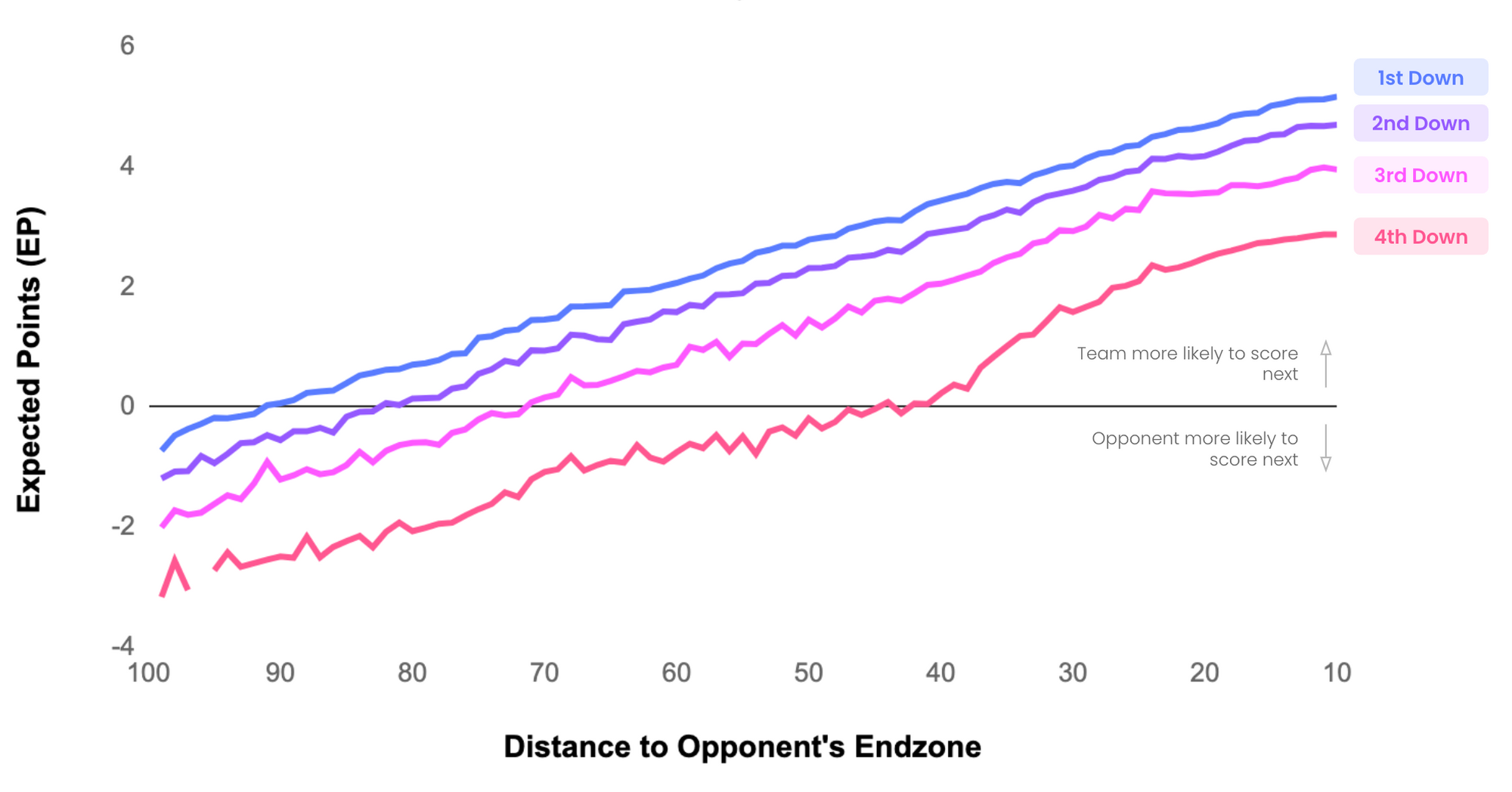
Expected Points (EP)

EP adds together the point value and probability of all potential outcomes of a possession. As teams approach their opponent’s endzone, the probability of scoring (Touchdowns and Field Goals) increases. Today, Expected Points models have evolved to account for significantly more game context. The models today are able to factor in things like down and distance, time remaining in the half, and the expected points the opponent gains once the ball is punted or a turned over is forced.

This unlocks insights into the relative values of downs at particular points on the field:

Expected Points Added (EPA)

EPA is the difference between a team’s Expected Points at the end of a play and their Expected Points at the beginning of a play. EPA essentially connects the dots between two game states. If a team ended the play with more Expected Points than they started, then EPA will be positive. If a team is left less likely to score at the end of the play, then EPA will be negative.

EPA is a great metrics that can be applied to a team's overall Offensive and Defensive EPA, but it can also be aggregated and averaged at the individual level to measure player performance. EPA is particularly useful when looking at individual QBs because QBs have a much higher influence over the outcome of a play relative to other skill positions like WR and RB.

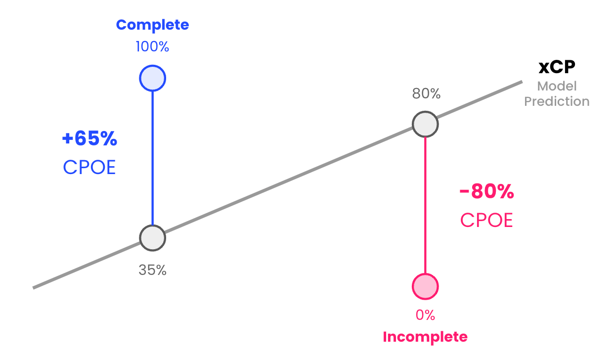
Completion Percentage Over Expected (CPOE)

CPOE measures how much higher (or lower) a QB’s completion percentage is relative to what we’d expect it to be based on the types of passes they attempted. CPOE is created through a machine learning model that predicts how likely a pass is to be completed (xCP) based on a variety of factors like the depth of the throw (short, medium, deep) and its location relative to the sideline (left, middle, right).

Over Expected metrics then, look at what actually happened on the play - was the pass complete or incomplete?  If a pass was completed, the actual completion percentage on that attempt would be 100%, and if it was incomplete, the actual completion percentage would be 0%. CPOE is then simply the difference between the observed result (CP) and the model’s expectation (xCP):

Yards After Catch Over Expected (YACOE)

YACOE is a metric best applied towards pass-catchers. Similar to CPOE, YACOE measures a player’s ability to gain more yards after the catch than what a league average player would be expected to do. Since WRs, TEs, and RBs are the primary pass-catching positions it makes sense that we would apply this metric to these positions. One other note is that OE metrics require different amounts of data to be accurate. For a WR's YACOE, it is recommended to include at least two season's worth of data to reach the same level of predictiveness as one season's worth of data for CPOE.

The reason YACOE requires more data relative to CPOE is because of the difference in volume. If a QB completes 30 pass attempts in a game, it is reasonable to assume that these passes will have been completed across a multitude different receivers. It's possible that one player will have only made one reception for the model to process. With less data, the model becomes more susceptible to inaccuracies.

Air Yards

Air yards are defined as the amount of yards the ball traveled in the air on a passing play, from line of scrimmage to contact point. If the quarterback throws the ball at the 25-yard line and the pass is caught at the 20-yard line, the amount of air yards on the pass was five yards.

Aggressiveness

I really like this statistic - here's a way to measure the aggressiveness of a QB by looking at a combination of different data points on 3rd down. In football, the ability to convert on 3rd down is important to a team's overall success because it gives offenses ability to sustain drives and control the time of possession.

By filtering our data to show pass plays where the air yards are greater than or equal to the number of yards to go, we can see which QB's are making the most aggressive throws.

Why is this aggressive? Well, the down and distance is a key variable. Despite the rise in 4th down attempts, 3rd down is still a pivotal down because an unsuccessful 3rd down often results in a punt. There are other factors that go into 3rd down decision making such as the score of the game, time remaining, timeouts remaining, and field position. Factoring in these additional variables is outside the scope of this metric but it might be something I explore at a later date.

Here is code for calculating aggressiveness in R:

aggressiveness <- data %>%
  group_by(passer_id) %>%
  filter(down == 3, play_type == "pass", ydstogo >= 5, ydstogo <= 10) %>%
  summarize(player_name = first(passer),
            team = first(posteam),
            total = n(),
            aggressive = sum(air_yards >= ydstogo, na.rm = TRUE),
            percentage = aggressive / total) %>%
  filter(total >= 50) %>%
  arrange(-percentage)

tibble(aggressiveness)